Context & Problem Statement
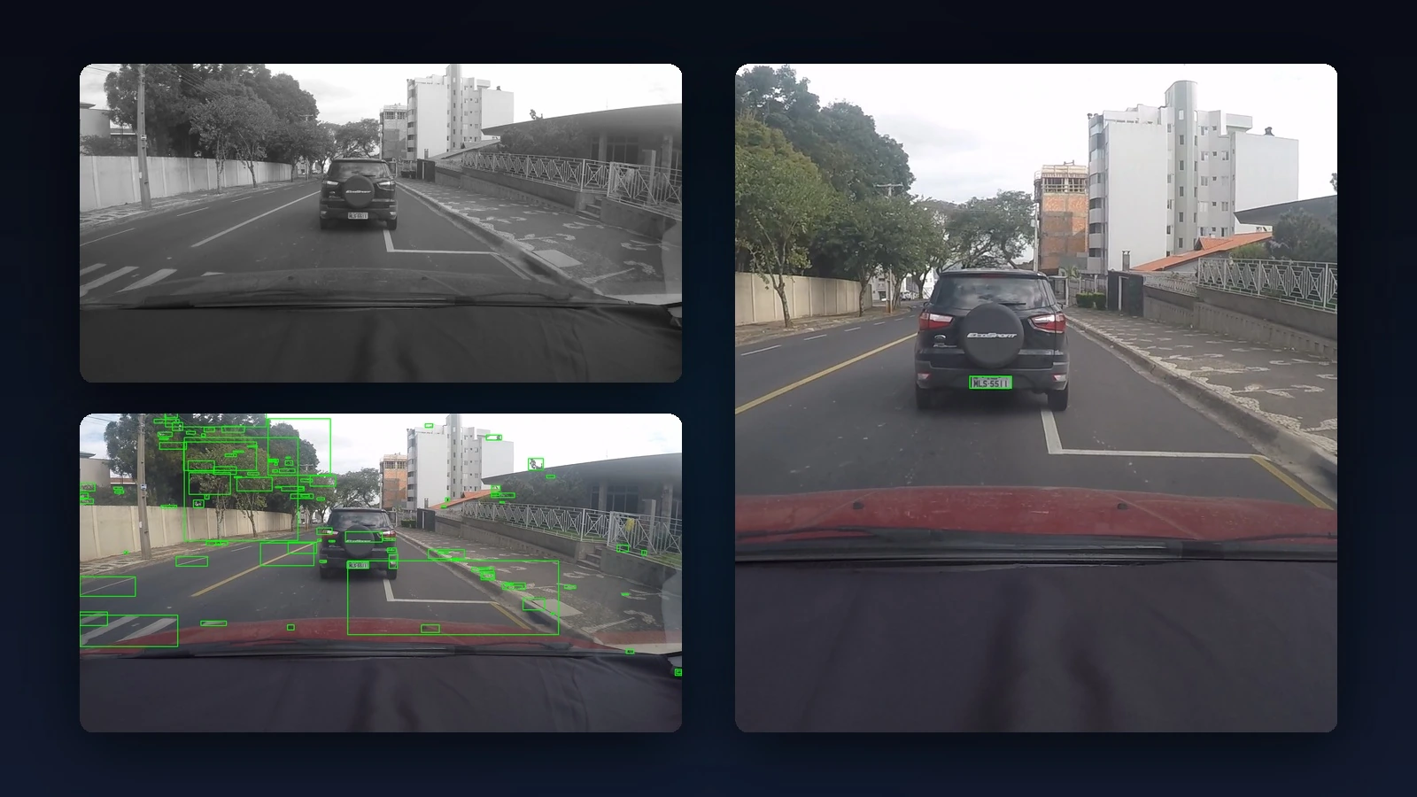
Automatic License Plate Recognition (ALPR) is a core building block of intelligent transportation systems and automated road access control. The goal of this project was to analyze high-resolution image streams and locate vehicle license plates with high precision, regardless of vehicle type or background environment.
Technical Challenges
- No-Deep-Learning Constraint: A major project constraint was to implement the entire pipeline without deep neural networks (no YOLO or heavy CNNs), relying strictly on classical computer vision and lightweight Machine Learning to guarantee complete explainability and a low memory footprint.
- High Resolution & Variability: Processing Full HD ($1920 \times 1080$) images featuring severe lighting variations (direct sunlight, rain, heavy shadows), tilted angles, and partial occlusions.
- Complex Plate Formats: Supporting both legacy Brazilian plates and new Mercosul standardized formats.
Workflow Overview
To solve this problem robustly, we structured the processing according to a 4-stage sequential pipeline:
- Preprocessing: Scale normalization and channel reduction.
- Candidate Generation (ROI): Multi-scale extraction of rectangular regions with a high probability of containing a plate.
- Feature Extraction: Numerical representation of each candidate using a vector of geometric descriptors and HOG.
- Classification & Validation: Evaluation of candidate regions by a Machine Learning model and selection of the top candidate.
Step-by-Step Algorithmic Pipeline
1. Image Preprocessing
The first step prepares the image to stabilize object dimensions and accelerate subsequent calculations:
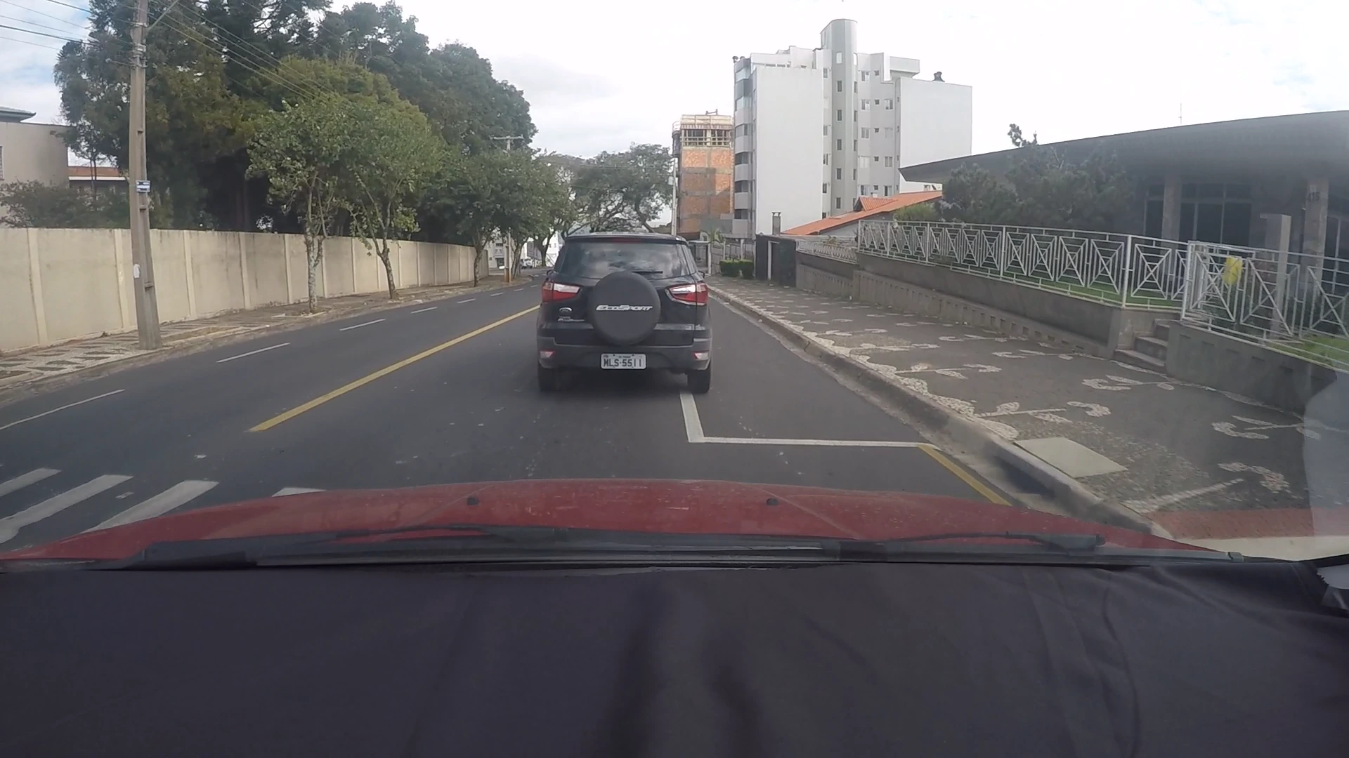
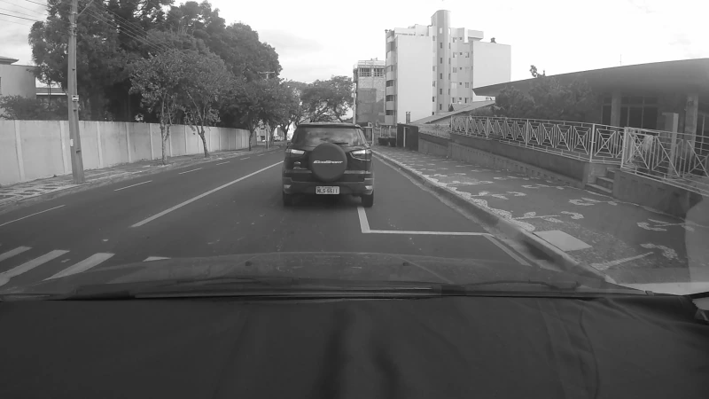
- Resizing to 800 pixels width while preserving aspect ratio to reduce computation time.
- Grayscale conversion to eliminate color and analyze luminance variations only.
| 1. Original Image | 2. Preprocessed Image |
|---|---|
 |
 |
2. Candidate Detection & Extraction (ROI)
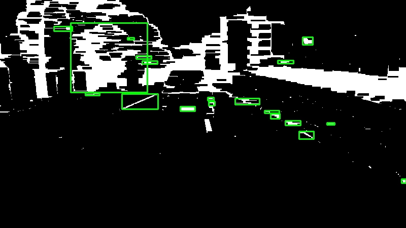
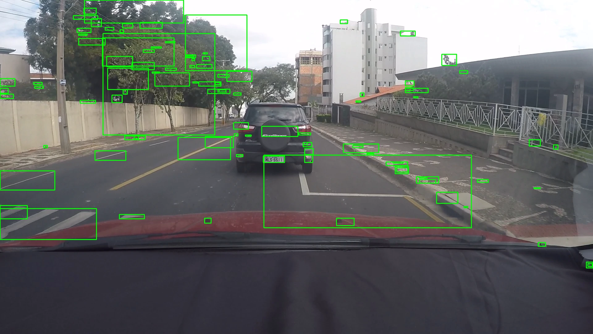
To avoid naively scanning the entire image, which would be extremely slow, we generate a small set of candidate Regions of Interest (ROI) by combining 3 complementary branches:
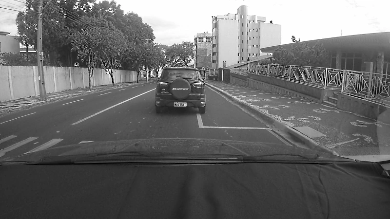
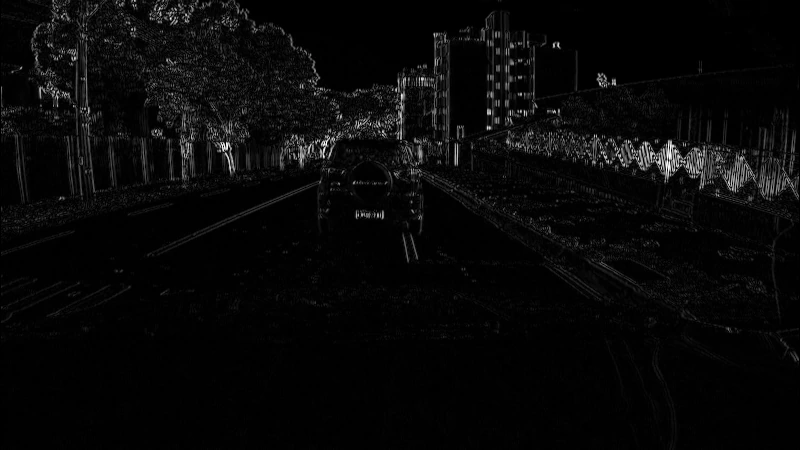
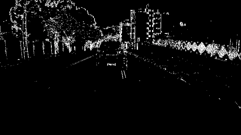
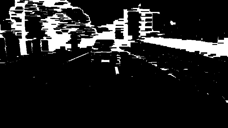
- Main Branch (Morphology + Sobel): Local contrast amplification of characters (MMLPF filter), followed by a vertical Sobel filter, Otsu thresholding, and morphological closing ($17 \times 3$).
- Oversampled Branch ($2\times$): Application of the same pipeline on the image enlarged to $2\times$ its size to capture very small or distant plates.
- Canny Branch: Adaptive edge detection based on the median image intensity.
Independent Geometric Filtering: Each branch immediately filters its own candidate regions based on their area ($50 \text{ px} \le \text{area} \le 40\,000 \text{ px}$) and aspect ratio ($1.0 \le w/h \le 8.0$) to eliminate obvious false candidates right away.
Steps of the Main Branch:
| 1: MMLPF Filter | 2: Vertical Sobel |
|---|---|
 |
 |
| 3: Otsu Thresholding | 4: Morphological Closing |
|---|---|
 |
 |
| 5: Extracted Candidates |
|---|
 |
3-Branch Fusion & NMS Deduplication
Similarly, the Oversampled Branch ($2\times$) and the Canny Branch extract and filter their own candidates. All candidate regions retained across all 3 branches are merged and deduplicated via Non-Maximum Suppression (NMS based on IoU) to eliminate overlaps.
3. Digital Signature (HOG & Geometry Descriptors)
Each retained candidate patch is cropped and resized to a fixed size of $64 \times 32$ pixels, then converted into a vector of 293 features:
- HOG Descriptor (288D): Histogram of Oriented Gradients computed across 32 cells of $8 \times 8$ pixels with 9 orientation bins and $L_2$ normalization.
- Geometric Metrics (5D): Aspect ratio, relative area, relative image position (X/Y), and edge density.
4. Classification & Final Localization
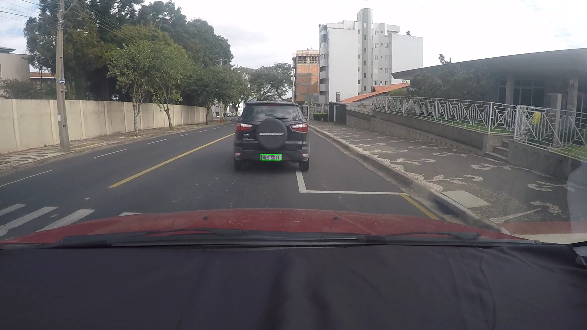
Each feature vector is fed to a Random Forest classifier (cv::ml::RTrees). The model assigns a confidence score to each candidate, and the region with the highest positive score is selected as the final plate.
Engineering Approach: From Python Prototype to C++17
The project evolved through two major phases:
1. Python Prototype (PoC)
Allowed rapid prototyping of the pipeline using scikit-learn and OpenCV Python, validating morphological filters, and training the classification model.
2. C++17 Port & Custom MyCV Module
To achieve the required real-time performance and move away from opaque OpenCV abstractions, we rewrote the pipeline in C++17 and designed a custom MyCV module containing:
- Dedicated grayscale conversion with weighted integer arithmetic.
- Custom 2D Sobel convolution with explicit memory and border handling.
- Native geometric operators.
Results & Benchmarks
Rigorous evaluation performed on the UFPR-ALPR test dataset (1,440 test images):
Inference Performance
| Implementation | True Positives (TP) | Precision | Recall | F1-Score | Average Time |
|---|---|---|---|---|---|
| Python | 955 | 0.8580 | 0.6632 | 0.7481 | 468.50 ms |
| C++17 (Optimized) | 963 | 0.8629 | 0.6687 | 0.7535 | 402.28 ms |
C++17 (MyCV) |
955 | 0.8504 | 0.6632 | 0.7452 | 583.67 ms |
Key Benchmark Takeaways
- Speed gain: Moving to C++17 reduced processing time by 14% (-66 ms per image).
- 92.85% perfect match between the Python prototype and the C++ implementation, confirming rewrite fidelity.
- Impact of SIMD optimization: The
MyCVversion (written in basic C++ loops without SIMD instructions) highlights the effectiveness of OpenCV’s vectorized routines (AVX2/NEON) for convolutions. - ML Training: Training time reduced from 3m46s to 2m48s thanks to better multi-core parallelization in C++ (441% CPU usage vs 201% in Python).