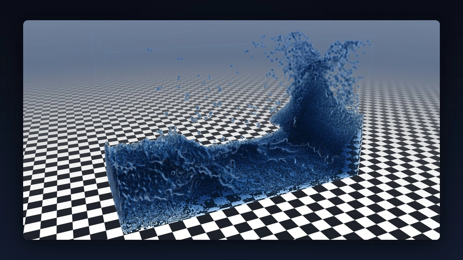
Context & Objectives
This project is a real-time 3D fluid simulation engine developed in C++20 and OpenGL 4.6 Core Profile, built for the Object-Oriented Programming and OpenGL (POGL) course at EPITA.
The goal was to design an engine executing two core graphics pillars in parallel:
- GPU Particle Physics Simulation via Smoothed Particle Hydrodynamics (SPH), fully computed by Compute Shaders, accelerated by 3D Spatial Hashing and a Bitonic GPU Sort in $O(N \log^2 N)$.
- Screen-Space Fluid Rendering (SSFR), a multi-pass pipeline transforming discrete particle clouds into a smooth continuous water surface featuring bilateral filtering, Beer-Lambert refraction, and Fresnel reflections.
Architecture: Data-Oriented Design GPU
The engine architecture follows Data-Oriented Design (DOD): all particle data resides in VRAM as Shader Storage Buffer Objects (SSBOs) in std430, eliminating PCIe transfer overhead between CPU and GPU during simulation frames.
The pipeline executes two distinct loops that chain together each frame:
| Phase | Responsibility | Tool |
|---|---|---|
| CPU | Inputs, SimSettings parameters | C++20, Dear ImGui |
| GPU — Physics | 7 Compute Shader passes | GLSL 4.60 |
| GPU — Rendering | 5 Graphics Shader passes (SSFR) | GLSL 4.60 |
The 8 SSBOs allocated in VRAM maintain positions, velocities, densities, spatial hashing, and rendering buffers — without ever transferring back to CPU during simulation.
Physics Engine: GPU SPH Simulation
The SPH method is a Lagrangian formulation of the Navier-Stokes equations: fluid is represented by discrete particles whose properties (density, pressure, viscosity) are estimated via weighted interpolation over neighboring particles using smoothing kernels.
Density & Pressure
The local density $\rho_i$ of a particle is the sum of contributions from neighboring particles $j$ within radius $h$:
$$\rho_i = \sum_{j} W_{\text{spiky2}}(\|\mathbf{r}_i - \mathbf{r}_j\|, h)$$A short-range secondary density $\rho_{\text{near}, i}$ (Spiky Power 3 kernel) strongly repels overly close particles, preventing excessive clustering. Pressure follows directly from deviation against target density $\rho_0$:
$$P_i = k \cdot (\rho_i - \rho_0), \qquad P_{\text{near}, i} = k_{\text{near}} \cdot \rho_{\text{near}, i}$$Forces & Integration
Pressure and viscosity forces are applied symmetrically (Newton’s 3rd Law):
$$\mathbf{F}_{\text{pressure}, i} = -\sum_{j} \frac{P_i + P_j}{2 \rho_j} \nabla W_{\text{spiky2}}(\|\mathbf{r}_{ij}\|, h) \cdot \hat{\mathbf{r}}_{ij}$$ $$\mathbf{F}_{\text{viscosity}, i} = \mu \sum_{j} (\mathbf{v}_j - \mathbf{v}_i) \cdot W_{\text{poly6}}(\|\mathbf{r}_{ij}\|, h)$$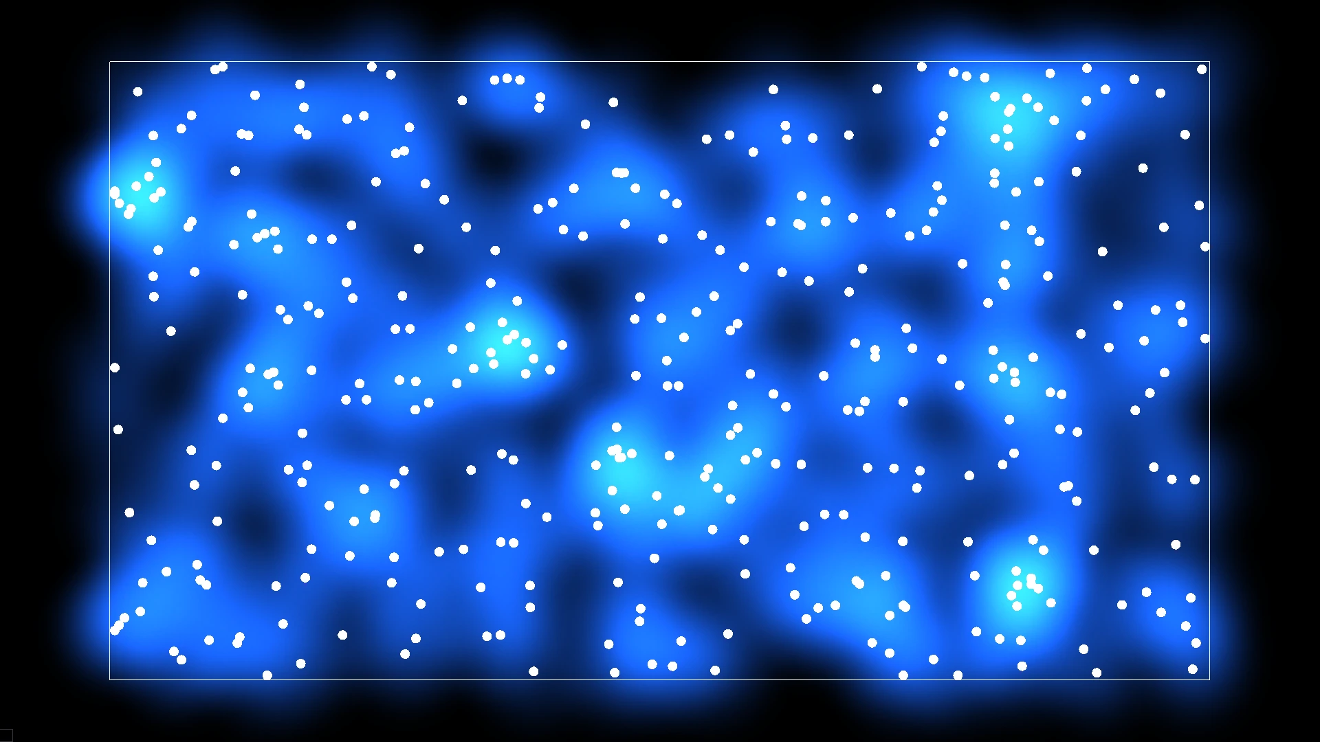
3D Spatial Hashing & Bitonic GPU Sort
Without optimization, neighbor search is $O(N^2)$, unfeasible for 75,000 particles. The 3D domain is subdivided into a regular grid (cells of size $h$) to reduce search complexity to $O(1)$.
Acceleration Pipeline (3 Compute Passes):
- Spatial Hashing: Each particle computes a hash of its 3D cell $\lfloor \mathbf{P}/h \rfloor$ using a prime-coefficient hash function.
- Bitonic GPU Sort: Pairs
(particleIndex, cellKey)are sorted in parallel on GPU in $O(\log^2 N)$ steps — zero CPU transfers required. - Index Offset Table: A fast pass identifies the starting index of each cell in the sorted array. Each particle then explores only its 27 adjacent 3D cells.
Rendering Pipeline: Screen-Space Fluid Rendering (SSFR)
Rendering particles as simple spheres results in a disjointed visual. Screen-Space Fluid Rendering converts point clouds into a continuous, realistic liquid surface across 5 sequential shader passes.
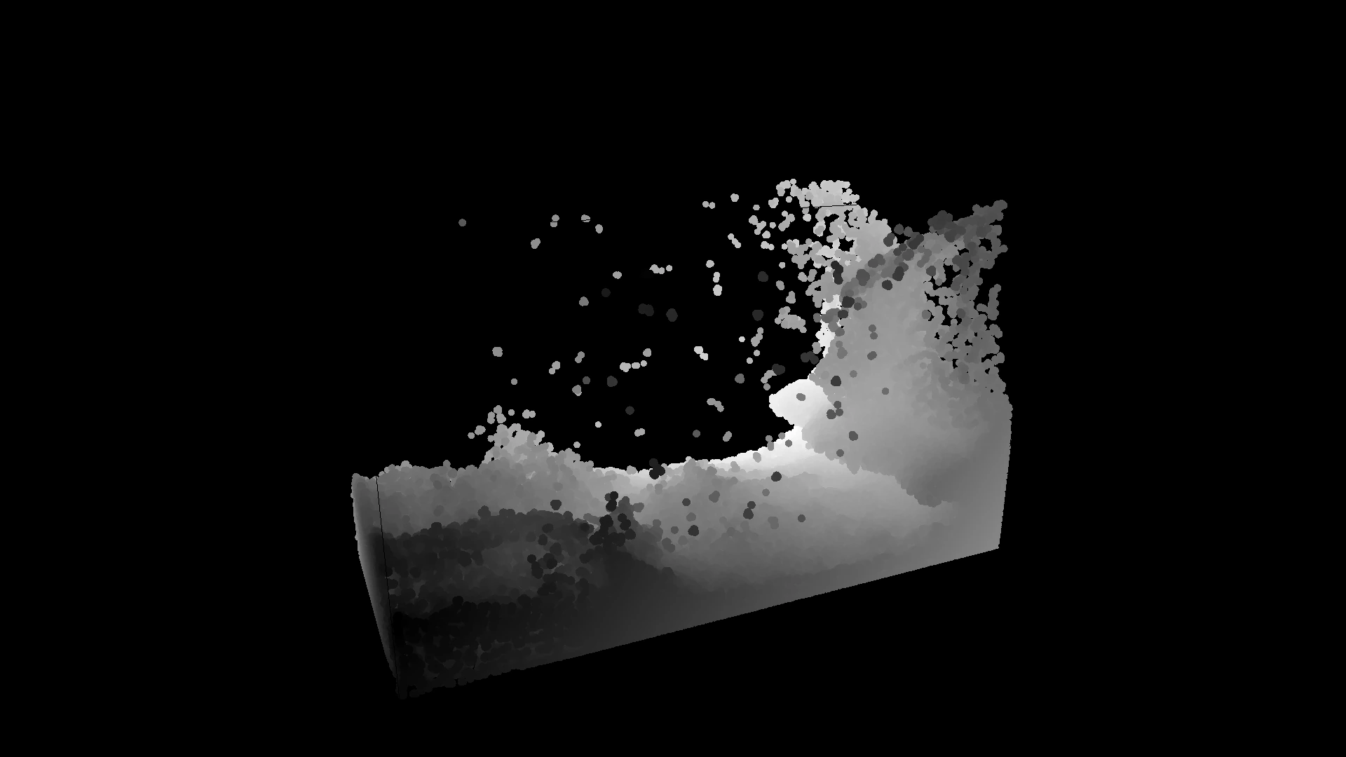
Pass 1 — Initial Depth Map
Each particle is rendered as a Point Sprite, projected into a 3D sphere in fluid_depth.frag. Fragments outside the sphere radius are discarded and exact depth $z_{\text{eye}}$ is saved into a GL_R32F texture.
Pass 2 — Adaptive Bilateral Filtering
A separable bilateral filter (two H/V passes) smoothes the depth map without blurring silhouette edges. Samples are weighted by both spatial distance and depth discrepancy:
$$W(i, j) = \exp\!\left(-\frac{\|\mathbf{x}_i - \mathbf{x}_j\|^2}{2 \sigma_s^2}\right) \cdot \exp\!\left(-\frac{|z_i - z_j|^2}{2 \sigma_r^2}\right)$$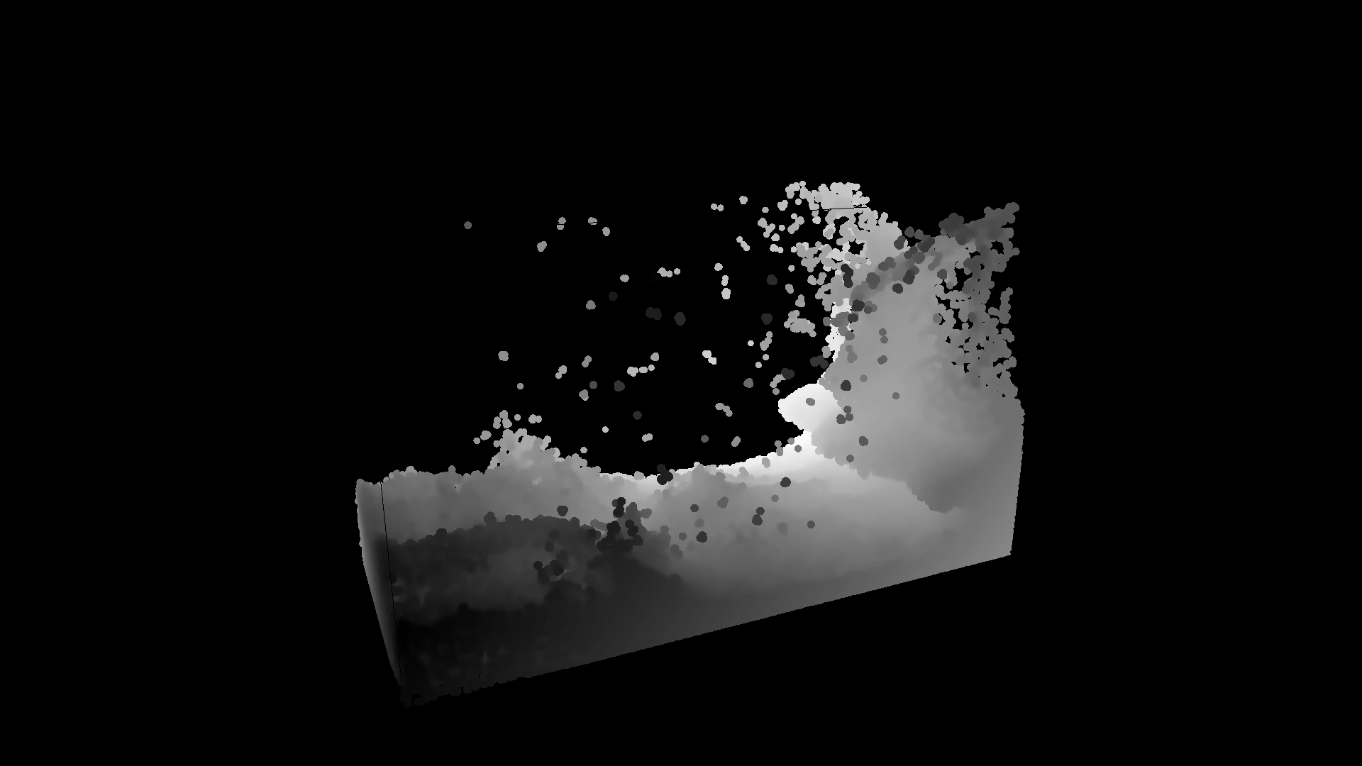
Pass 3 — Screen-Space 3D Normal Reconstruction
From smoothed depth $z(u, v)$, the 3D position $\mathbf{P}(u, v)$ is reconstructed per pixel. The normal field is derived via the cross product of partial derivatives:
$$\mathbf{N} = \text{normalize}\!\left( \frac{\partial \mathbf{P}}{\partial x} \times \frac{\partial \mathbf{P}}{\partial y} \right)$$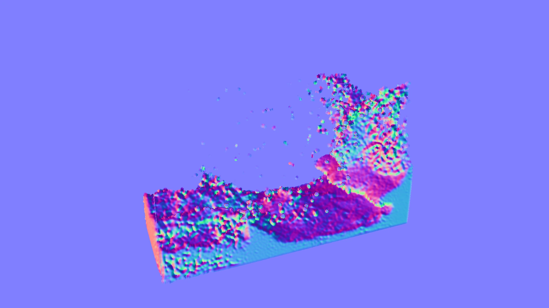
Pass 4 — Thickness & Optical Absorption (Beer-Lambert)
Traversed water thickness is accumulated using additive blending (GL_ONE, GL_ONE). Chromatic attenuation follows the Beer-Lambert law:
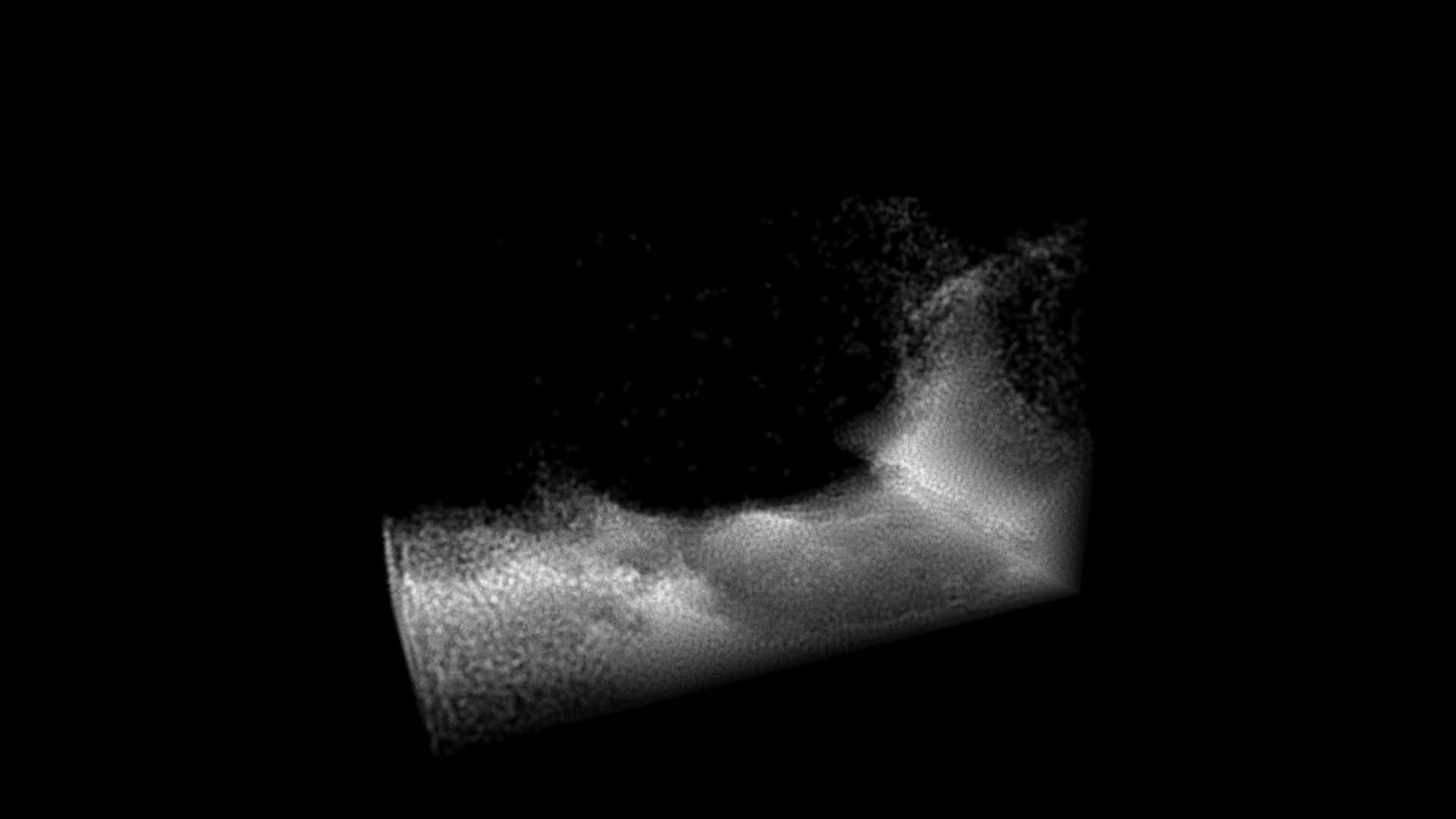
Pass 5 — Final Composition: Refraction & Fresnel Reflections
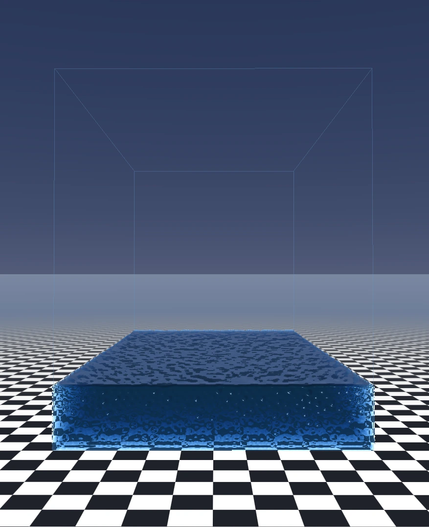
The final pass combines all buffers:
- Refraction: UV offset proportional to surface normal ($\text{UV}_{\text{refracted}} = \text{UV} + \mathbf{N}_{xy} \cdot s_{\text{refraction}}$).
- Fresnel Reflections (Schlick): $F(\theta) = R_0 + (1 - R_0)(1 - \cos\theta)^p$ — water becomes reflective at grazing angles.
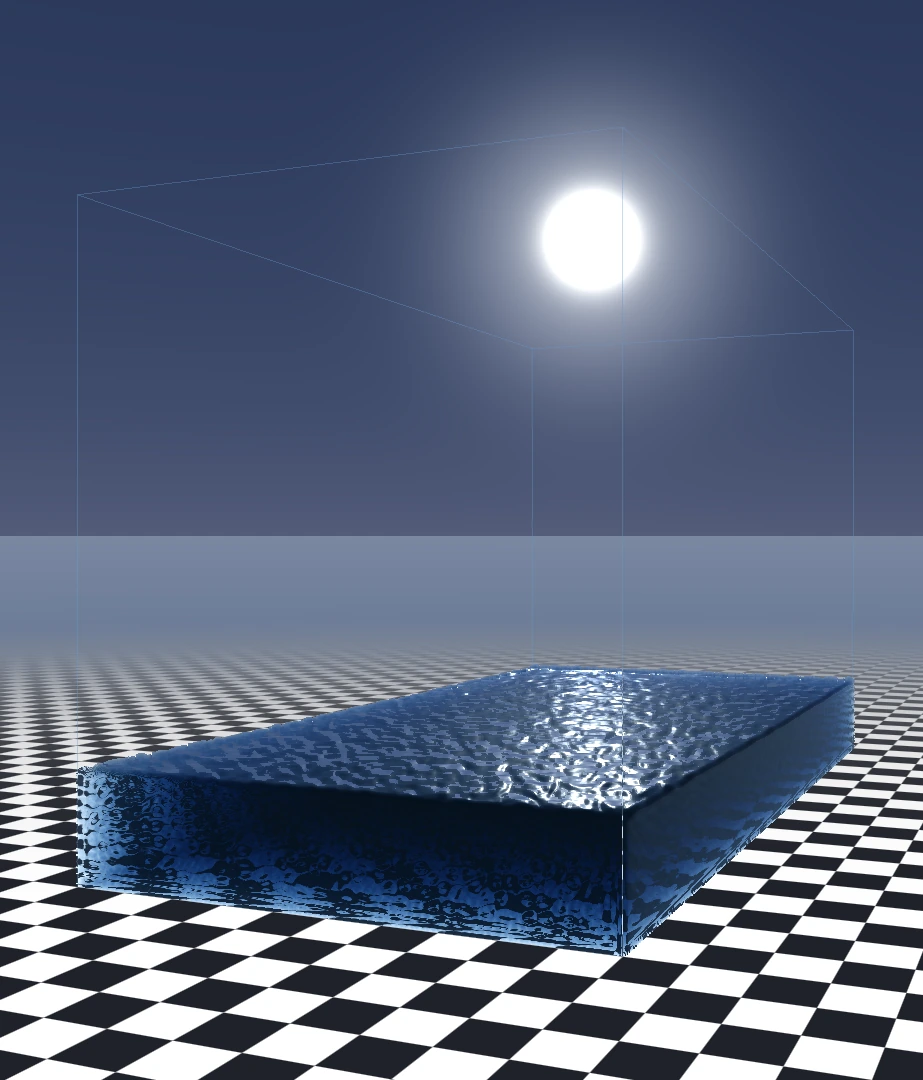
- Procedural Sky & Specular Highlights: Blended according to Fresnel coefficient between absorbed refraction and sky/sun reflection.
| Pass 5: Global Reflection & Refraction | Pass 5: Sun Specular Highlights |
|---|---|
 |
 |
Interactive UI & Controls
The application embeds Dear ImGui to allow dynamic real-time tuning of parameters: particle count, gravity $g$, stiffness $k$, viscosity $\mu$, water color, absorption, Fresnel power, and bilateral blur radius.
The camera is orbital (left click + drag) with scroll zoom.
GPU Optimizations
- Workgroup of 256 threads per Compute group, optimized for NVIDIA SM (Warps) and AMD (Wavefronts) occupancy.
- Explicit memory barriers (
GL_SHADER_STORAGE_BARRIER_BIT) ensuring data consistency between physics and rendering passes. - Resizable FBOs dynamically adapting to window resize events without unnecessary allocations.
- Zero CPU ↔ GPU transfers during simulation: physics is entirely computed and consumed in VRAM.